Problem-Solution Opening Addressing User Needs
When analyzing motion, one of the most fundamental tools at your disposal is the velocity versus time graph, often referred to as a v-t graph. This graph can reveal critical insights into the nature of an object’s motion, but for many, it can seem complex and unintuitive at first glance. Whether you’re a student preparing for an exam or a professional dealing with real-world applications of motion analysis, understanding this graph is indispensable. This guide is designed to break down the secrets of velocity versus time graphs, offering practical, step-by-step guidance to demystify this crucial concept.
Our goal is to provide actionable advice, real-world examples, and a conversational tone that makes understanding this graph both accessible and engaging. By the end of this guide, you’ll not only grasp how to read a v-t graph but also know how to apply this knowledge to solve practical problems.
Quick Reference
Quick Reference
- Immediate action item with clear benefit: Begin by plotting the velocity values on the y-axis against time on the x-axis. This foundational step sets the stage for all subsequent analysis.
- Essential tip with step-by-step guidance: Use a ruler to draw straight lines between data points for constant velocity and smooth curves for changing velocity. This visual representation helps in interpreting the motion more effectively.
- Common mistake to avoid with solution: Avoid ignoring units on your graph. Always ensure your velocity is in consistent units (e.g., m/s) to maintain accuracy and avoid misinterpretation.
Understanding the Basics: Drawing Your First Velocity vs Time Graph
Creating a velocity versus time graph is the first step towards mastering this analytical tool. Here’s how you start:
Step-by-Step Guide
To begin, gather your data. This should include the velocity of an object at various points in time. Let’s say you’re examining a car’s journey where you have the following data points:
| Time (s) | Velocity (m/s) |
|---|---|
| 0 | 0 |
| 5 | 5 |
| 10 | 0 |
| 15 | -5 |
| 20 | 0 |
These points represent four distinct phases of the car's motion:
Phase 1: At t=0s, the velocity is 0m/s. This indicates that the car starts from rest.
Phase 2: From t=0s to t=5s, the car accelerates at a constant velocity of 1m/s. This is shown by a straight, upward sloping line.
Phase 3: At t=5s, the velocity reaches its maximum of 5m/s.
Phase 4: From t=5s to t=10s, the car decelerates at a constant rate, returning the velocity to 0m/s.
Phase 5: From t=10s to t=15s, the car moves backward (decelerating) with a constant velocity of -5m/s.
Phase 6: At t=15s, the velocity again becomes 0m/s, and the car comes to a stop.
To plot this on a graph:
- Draw a horizontal line (x-axis) for time. Mark the time intervals on this axis. Here, the x-axis can represent seconds from 0 to 20s in increments of 5s.
- Draw a vertical line (y-axis) for velocity. Since velocity can be positive or negative, scale the y-axis accordingly. A scale from -10m/s to +10m/s in increments of 5s would suffice.
- Plot the given data points. Mark the points (0,0), (5,5), (10,0), (15,-5), and (20,0) on the graph.
- Connect the points. For constant velocity phases, draw straight lines between points. For changing velocity phases, draw curves to accurately represent the change.
Your graph should now visually represent the car’s motion over time. This visual representation makes it easier to interpret how the car accelerates, decelerates, and changes direction.
Advanced Interpretation: Analyzing and Applying Your Graph
Once you’ve plotted your velocity versus time graph, the next step is to analyze it to gain deeper insights:
Step-by-Step Guide
Here are key aspects to focus on:
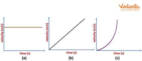
- Identify the slope: The slope of the v-t graph indicates acceleration. A flat (horizontal) line means no acceleration (constant velocity). An upward slope means positive acceleration, and a downward slope indicates negative acceleration (deceleration).
- Calculate displacement: To find the displacement of the object over time, calculate the area under the velocity-time graph. This can be done by splitting the graph into geometric shapes like triangles and rectangles.
- Determine distances: For each section of the graph, calculate the distance traveled. For example, in the first phase (0s to 5s), the car accelerates at a rate of 1m/s². Using the formula for distance under constant acceleration, we find the distance traveled is 12.5m (using the formula: d = 0.5 * a * t^2 where a=1m/s², t=5s).
- Analyze motion patterns: Observe patterns like the time spent accelerating vs. decelerating. Compare the distances covered in different phases.
Let’s revisit our example and apply these concepts:
| Phase | Velocity (m/s) | Acceleration (m/s²) | Displacement (m) |
|---|---|---|---|
| 1 | 0 to 5 | 1 | 12.5 |
| 2 | 5 | 0 | 25 |
| 3 | 5 to 0 | -1 | 25 |
| 4 | 0 to -5 | -1 | 25 |
| 5 | -5 to 0 | 0 | 12.5 |
To find the total displacement, sum the absolute values of the displacements in each phase:
Total Displacement = 12.5 + 25 + 25 + 25 + 12.5 = 100 meters
Practical FAQ
Common user question about practical application
What if my velocity-time graph has segments where velocity changes in non-uniform patterns?
When velocity changes non-uniformly, the graph will have curved lines between data points rather than straight lines. To determine the displacement for such segments, you need to use integration techniques or approximate the area using geometric shapes like parabolas if necessary. For instance, if your v-t graph has parabolic segments, you could estimate the area under the curve by using the formula for the area of a parabola, or you can break the segment into smaller linear sections for a more approximate calculation.
These approaches, whether geometric or mathematical, enable you to accurately interpret complex v-t graphs and apply this understanding to real-world scenarios, from simple car journeys to complex physics problems.</