Understanding the logistic growth curve is crucial for various fields, from biology to economics, as it models how systems grow rapidly at first and then level off as they approach a certain limit. This guide will walk you through the practical aspects of understanding and applying logistic growth models, providing actionable advice to help you master this concept effectively.
Problem-Solution Opening Addressing User Needs
Logistic growth models can often be daunting due to their complex mathematical nature. If you're struggling to understand how they work or how to apply them to real-world data, you're not alone. Many people find the initial theoretical concepts challenging to grasp and subsequently find it hard to translate these concepts into practical applications. However, by breaking down the logistic growth curve into simpler, digestible parts and focusing on practical examples, you can unlock its potential and apply it to a wide range of scenarios. This guide is designed to demystify the logistic growth curve, offering step-by-step guidance and actionable advice to help you understand its key elements and leverage it to make informed decisions in your field of interest.
Quick Reference
Quick Reference
- Immediate action item: Plot a sample logistic growth curve to visualize its shape and key characteristics.
- Essential tip: Start with simple linear growth models before transitioning to logistic curves to build a foundational understanding.
- Common mistake to avoid: Confusing the logistic curve with exponential growth; the logistic curve peaks and levels off, unlike exponential growth which continues to rise.
Understanding the Logistic Growth Curve
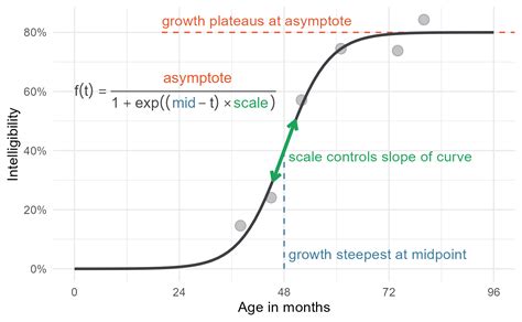
The logistic growth curve is an S-shaped curve that describes a process of growth beginning with a slow start, accelerating, and then leveling off as the process reaches its carrying capacity.
The general form of the logistic growth equation is:
N(t) = K / (1 + (K - N0) / N0 * e^(-rt))
Where:
- N(t) is the quantity at time t
- K is the carrying capacity
- N0 is the initial quantity
- r is the growth rate constant
- t is time
- e is the base of the natural logarithm
This equation helps you predict how a population or system will grow over time, factoring in a limited carrying capacity.
Detailed How-To Section: Creating a Logistic Growth Curve
Step-by-Step Guide to Creating a Logistic Growth Curve
Creating a logistic growth curve involves several steps. Here’s how you can do it:
Step 1: Understand the Key Variables
Before you start plotting your logistic growth curve, ensure you understand the key variables involved:
- Carrying Capacity (K): This is the maximum value the growth can reach.
- Initial Population (N0): This is the starting value before growth begins.
- Growth Rate ®: This is how quickly the population grows initially.
Step 2: Gather Data
To create a logistic growth curve, you need data that follows an S-shaped growth pattern. For example, you might use data from a biological population study where you have measurements of population size over time.
Step 3: Plotting the Curve
Using software like Excel or Python, you can plot the curve. Here’s a basic guide:
In Python, you can use the following script:
import numpy as np
import matplotlib.pyplot as plt

# Define the logistic function
def logistic(t, K, N0, r):
    return K / (1 + (K - N0) / N0 * np.exp(-r * t))

# Parameters
K = 1000  # carrying capacity
N0 = 10  # initial population size
r = 0.4  # growth rate

# Time points
t = np.linspace(0, 50, 100)

# Calculate population
N = logistic(t, K, N0, r)

# Plotting
plt.plot(t, N, label='Logistic Growth')
plt.xlabel('Time')
plt.ylabel('Population')
plt.title('Logistic Growth Curve')
plt.legend()
plt.show()
This script defines the logistic function, sets parameters, calculates the population for each time point, and plots the logistic growth curve.
Step 4: Analyzing the Curve
Once the curve is plotted, you can analyze it to understand where it’s accelerating and where it’s leveling off. The initial part of the curve is steep, indicating rapid growth, while the latter part levels off as the system approaches its carrying capacity.
Step 5: Making Predictions
Using your logistic growth curve, you can make predictions about future population sizes within the system’s carrying capacity. This is especially useful in fields like biology, economics, and resource management.
Practical FAQ
How can I tell if my data follows a logistic growth pattern?
To determine if your data follows a logistic growth pattern, look for an S-shaped curve. You can plot your data and see if it initially grows rapidly and then levels off. Additionally, check if the rate of change starts to decrease as your system approaches its maximum capacity (carrying capacity). You can also fit a logistic curve to your data and see if it provides a good fit. Using software like Python with the SciPy library can help you fit a logistic curve and evaluate its goodness of fit.
Can logistic growth models predict real-world scenarios accurately?
Logistic growth models can be quite accurate in predicting real-world scenarios when the underlying assumptions are valid and the data is properly collected. For instance, in biology, logistic models can accurately predict the growth of populations within limited resource environments. However, the accuracy depends on how well the data represents the real-world scenario and the assumptions of the model. It’s crucial to validate the model against real data and possibly use additional data collection to refine the model’s predictions.
What are some common pitfalls when using logistic growth models?
One common pitfall is underestimating the carrying capacity, which can lead to overestimating future growth. Another issue is not properly accounting for variability in the data, which can result in misleading predictions. It’s important to use robust statistical methods to estimate the parameters of the logistic model and validate the model with real-world data. Additionally, avoid using the logistic model for processes that do not inherently have a limiting factor; this will result in inaccurate predictions.
This comprehensive guide aims to help you master the logistic growth curve, providing practical examples and actionable advice to ensure you can apply this concept effectively in your specific field. By understanding and implementing the logistic growth model, you can gain valuable insights into the dynamics of growth processes and make informed decisions based on predictive analytics.