Understanding and mastering the Cobb-Douglas function is critical for anyone involved in economic analysis, business strategy, or advanced production planning. The Cobb-Douglas production function is a cornerstone model in economics, encapsulating the relationship between inputs (like labor and capital) and the output produced. This guide aims to demystify the function, providing you with practical insights and step-by-step advice on how to implement and leverage this powerful economic tool.
Addressing Your Need for Cobb-Douglas Mastery
For businesses and economists, the Cobb-Douglas function often appears intimidating due to its mathematical complexity. However, mastering this function can dramatically enhance your understanding of how productivity is shaped by different factors. Whether you are analyzing the efficiency of production processes or aiming to optimize resource allocation, a solid grasp of this function is invaluable. This guide will break down the function into digestible parts, equipping you with the knowledge to apply it effectively in real-world scenarios.
Quick Reference
Quick Reference
- Immediate action item with clear benefit: Start by plotting your production data to see if it aligns with a Cobb-Douglas relationship. If it does, you can use this function to predict future outputs and identify areas for improvement.
- Essential tip with step-by-step guidance: Use logarithmic transformation on your data to linearize the Cobb-Douglas function, making it easier to estimate parameters using simple regression techniques.
- Common mistake to avoid with solution: Don’t overlook the role of diminishing returns. When using this function, ensure you account for diminishing marginal returns by keeping your input levels balanced.
Understanding the Cobb-Douglas Function
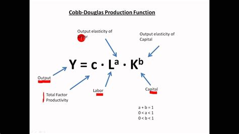
The Cobb-Douglas function is typically expressed as:
Q = A * L^α * K^β
Where:
- Q represents the output quantity.
- L is the amount of labor used.
- K is the amount of capital used.
- A is a constant that reflects technological level and efficiency.
- α and β are the output elasticities of labor and capital, respectively.
This function suggests that output (Q) is a function of labor (L) and capital (K), raised to certain powers that reflect their respective contributions. To practically apply this model:
Step-by-Step Application
To apply the Cobb-Douglas function in a practical setting, follow these detailed steps:
Step 1: Data Collection
Collect data on your production processes. You’ll need the amount of labor, capital, and the corresponding output levels for various points in time. For example:
| Time | Labor (L) | Capital (K) | Output (Q) |
|---|---|---|---|
| 1 | 50 | 100 | 500 |
| 2 | 60 | 120 | 620 |
| 3 | 70 | 130 | 700 |
These data points will help you build your model.
Step 2: Linearizing the Function
To estimate the parameters of the Cobb-Douglas function, you need to linearize it. This is done by taking the natural logarithm of both sides:
ln(Q) = ln(A) + α * ln(L) + β * ln(K)
Now, you have a linear equation that can be estimated using regression analysis.
Step 3: Regression Analysis
Use statistical software or a spreadsheet to perform a regression analysis on your transformed data. This will give you estimates for ln(A), α, and β. For example, if your regression results show:
| Variable | Coefficient | Standard Error |
|---|---|---|
| ln(A) | 3.5 | 0.1 |
| α * ln(L) | 0.8 | 0.05 |
| β * ln(K) | 0.6 | 0.04 |
You can exponentiate the coefficient for ln(A) to get the constant A, which is e^3.5 ≈ 33.1.
Step 4: Interpretation
Interpreting your results involves understanding the elasticity of output with respect to labor and capital. An elasticity of 0.8 for labor means that a 1% increase in labor leads to approximately 0.8% increase in output. Similarly, for capital, an elasticity of 0.6 means a 1% increase in capital leads to a 0.6% increase in output.
Step 5: Application
Now that you have your Cobb-Douglas function, you can use it to predict future outputs. For instance, if you plan to increase labor to 80 and capital to 150:
Q = 33.1 * (80)^0.8 * (150)^0.6 ≈ 1100
This calculation helps you forecast potential output levels, aiding in strategic decision-making.
Practical FAQ
How can I ensure my Cobb-Douglas model is accurate?
Accuracy in the Cobb-Douglas model hinges on high-quality data and proper regression analysis:
- Data Quality: Ensure your data on labor, capital, and output is precise and covers a broad range of production conditions.
- Data Transformation: Correctly transform your data by taking natural logs, ensuring the regression analysis aligns with the Cobb-Douglas form.
- Model Validation: Test your model by comparing predicted outputs with actual outcomes to check for significant deviations.
- Consider External Factors: Sometimes, external variables like technology changes, market conditions, or regulatory shifts can affect your model’s predictions. Including these as dummy variables in your regression can improve accuracy.
Regularly updating your model with new data also helps maintain its accuracy over time.
Mastering the Cobb-Douglas function will provide a solid foundation for optimizing productivity and improving economic efficiency in your business or research project. By following the steps outlined in this guide, you’ll be well-equipped to implement this model and leverage its insights for strategic advantage.